boxplot(airquality$Ozone)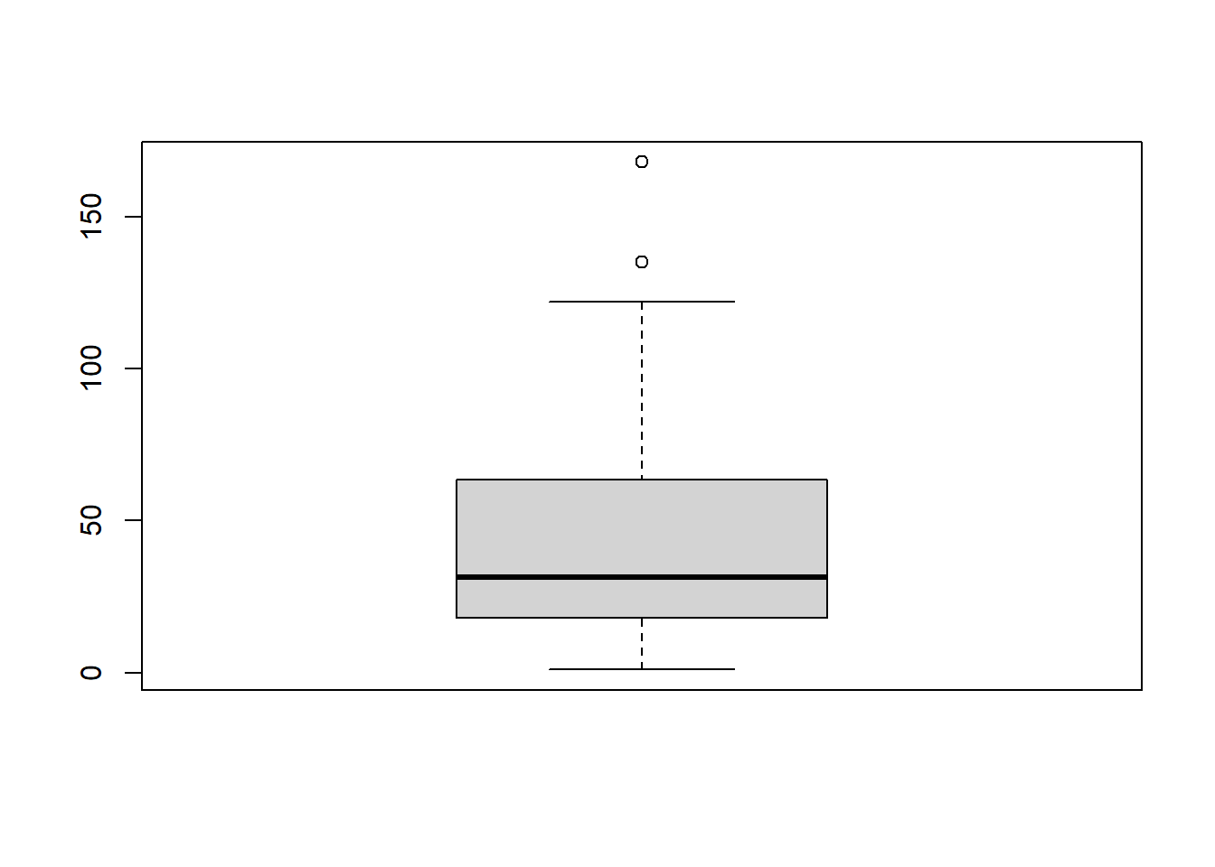
R in statistics
👉🏻Click to enter the ENV222 note section
1.
The distribution is shown in Figure @ref(fig:box).
boxplot(airquality$Ozone)
2.
rticles
3.
plot(1,
     type = 'n',
     axes = FALSE,
     xlab = expression(NH[3] * " (" * mu* "mol m"^-3 * ")"),
     ylab = '')
dtf <- c('1', '2', '3')
library(latex2exp)
plot(dtf, pch = 16, las = 1,
     xlab = TeX('$NH_3$ ($\\mu$mol m$^{-3}$)'),
     xaxt = "n", yaxt ="n",
     line=0.4)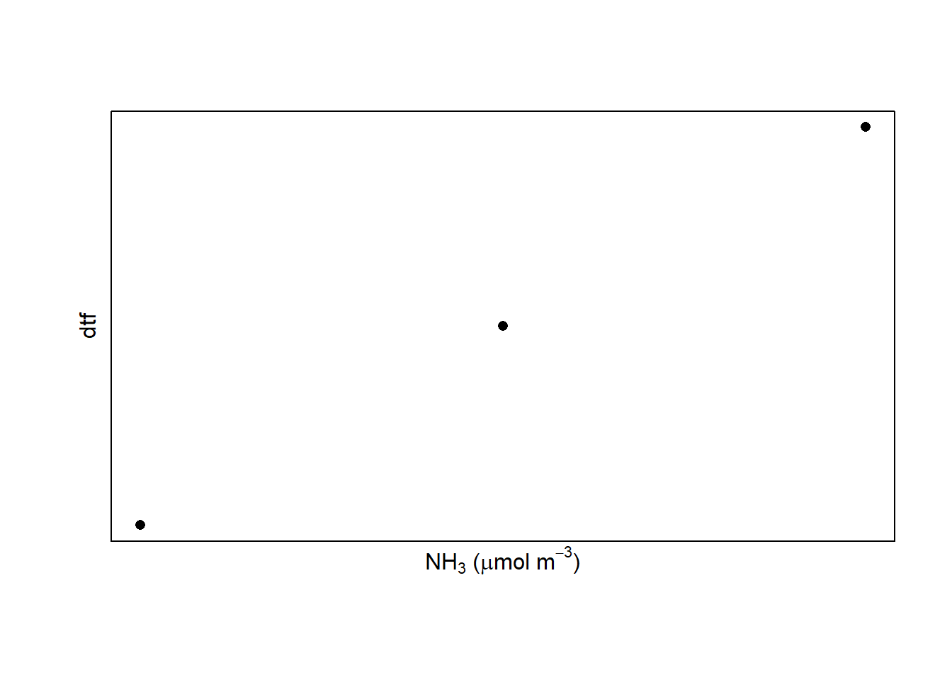
mymat <- matrix(c(1, 2, 3, 0), nrow = 2)
layout(mymat, widths = c(4, 1), heights = c(2, 1))  # Set the ratio between widths and heights
plot(iris$Sepal.Length, iris$Sepal.Width, pch=20, xlab='Sepal Length (cm)', ylab='Sepal Width (cm)', las=1)
boxplot(iris$Sepal.Length, pch=20, las=1, horizontal=T)
boxplot(iris$Sepal.Width, pch=20, las=2)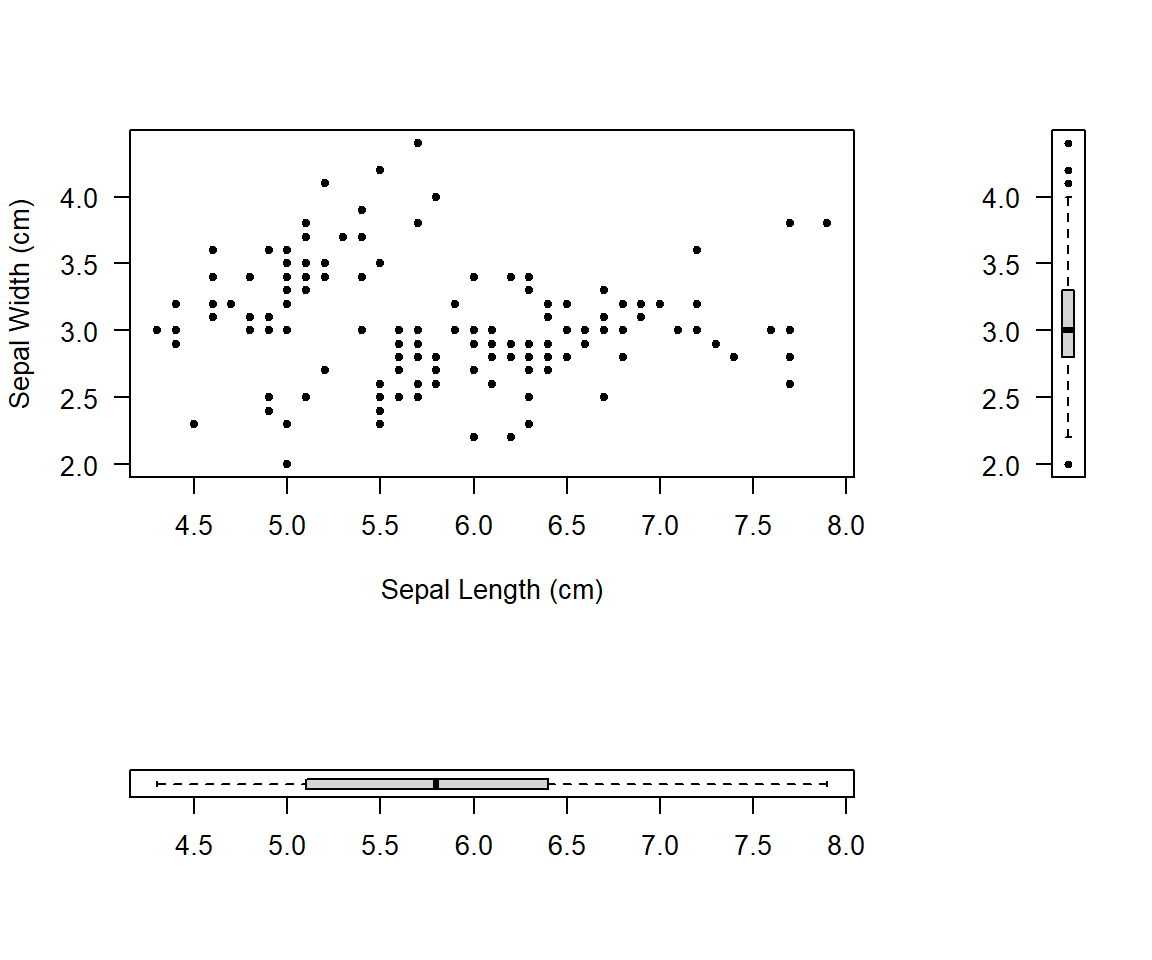
x <- 'pack my box with five dozen liquor jugs'
xsingle <- strsplit(x, split = "")[[1]]
xsingle <- xsingle[xsingle != " "]
length(xsingle)
[1] 32mytab <- table(xsingle)
names(mytab[mytab == max(mytab)])[1] "i" "o"library(dplyr)
x <- "pack my box with five dozen liquor jugs"
char_freq <- gsub(" ", "", x) |>
strsplit("") |>
table() |>
data.frame() |>
arrange(desc(Freq))
head(char_freq, 5) Var1 Freq
1 i 3
2 o 3
3 e 2
4 u 2
5 a 1xword <- strsplit(x, " ")[[1]]
xword[which.max(nchar(xword))][1] "liquor"gsub('five', '5', x)[1] "pack my box with 5 dozen liquor jugs"[1] "English_United States.1252"sum(diff(mydata$date) != 1)[1] 0mydata$year <- as.integer(format(mydata$date, '%Y'))mydata$month <- format(mydata$date, '%B')mydata$weekday <- format(mydata$date, '%A')Result:
mydata# A tibble: 65,533 × 13
date ws wd nox no2 o3 pm10 so2 co pm25
<dttm> <dbl> <int> <int> <int> <int> <int> <dbl> <dbl> <int>
1 1998-01-01 00:00:00 0.6 280 285 39 1 29 4.72 3.37 NA
2 1998-01-01 01:00:00 2.16 230 NA NA NA 37 NA NA NA
3 1998-01-01 02:00:00 2.76 190 NA NA 3 34 6.83 9.60 NA
4 1998-01-01 03:00:00 2.16 170 493 52 3 35 7.66 10.2 NA
5 1998-01-01 04:00:00 2.4 180 468 78 2 34 8.07 8.91 NA
6 1998-01-01 05:00:00 3 190 264 42 0 16 5.50 3.05 NA
7 1998-01-01 06:00:00 3 140 171 38 0 11 4.23 2.26 NA
8 1998-01-01 07:00:00 3 170 195 51 0 12 3.88 2.00 NA
9 1998-01-01 08:00:00 3.36 170 137 42 1 12 3.35 1.46 NA
10 1998-01-01 09:00:00 3.96 170 113 39 2 12 2.92 1.20 NA
# ℹ 65,523 more rows
# ℹ 3 more variables: year <int>, month <chr>, weekday <chr>1.
C
2.
B
3.
Wilcoxon Rank-Sum test
4.
5.
There are no duplicated values, because the rank are all int
rank(c(13.31, 13.67, 12.805, 13.1, 13.39, 12.375, 11.58, 14.58, 12.029, 13.69)) [1] 6 8 4 5 7 3 1 10 2 9rank(c(14.14, 12.54, 15.63, 13.66, 15.51, 13.23, 13.25, 15.2, 14.18, 14.53)) [1] 5 1 10 4 9 2 3 8 6 76.
Test statistic value: W = 23
dtf <- data.frame(City_A = c(13.31, 13.67, 12.805, 13.1, 13.39, 12.375, 11.58, 14.58, 12.029, 13.69),
                  City_B = c(14.14, 12.54, 15.63, 13.66, 15.51, 13.23, 13.25, 15.2, 14.18, 14.53))
test <- wilcox.test(dtf$City_A, dtf$City_B, conf.int=TRUE)
test$statistic
W
23 7.
Critical values of 95 percent confidence interval: 24, 76
dtf <- data.frame(conc = c(13.31, 13.67, 12.805, 13.1, 13.39, 12.375, 11.58, 14.58, 12.029, 13.69, 14.14, 12.54, 15.63, 13.66, 15.51, 13.23, 13.25, 15.2, 14.18, 14.53),
                  city = c(rep("A", 10), rep("B", 10)))
m <- sum(dtf$city == "A")
n <- sum(dtf$city == "B")
U_critical  <- qwilcox(c(0.025, 0.975), m, n)
U_critical
[1] 24 76dtf <- data.frame(City_A = c(13.31, 13.67, 12.805, 13.1, 13.39, 12.375, 11.58, 14.58, 12.029, 13.69),
City_B = c(14.14, 12.54, 15.63, 13.66, 15.51, 13.23, 13.25, 15.2, 14.18, 14.53))
m <- nrow(dtf)
n <- nrow(dtf)
U_critical <- qwilcox(c(0.025, 0.975), m, n)
U_critical[1] 24 76U <- 23
m <- 10
n <- 10
curve(dwilcox(x, m, n), from = 0, to = 100, n = 101, ylab = 'Probability distribution density', las = 1, type = 'S', ylim = c(0, 0.031))
abline(h = 0)
segments(x0 = c(U, U_critical), y0 = 0, x1 = c(U, U_critical), y1 = dwilcox(c(U, U_critical), m, n), col = c('blue', 'red', 'red'))
legend('topright', legend = c('Distribution curve', 'Critical values', 'U score'), col = c('black', 'red', 'blue'), lty = 1,cex=0.7)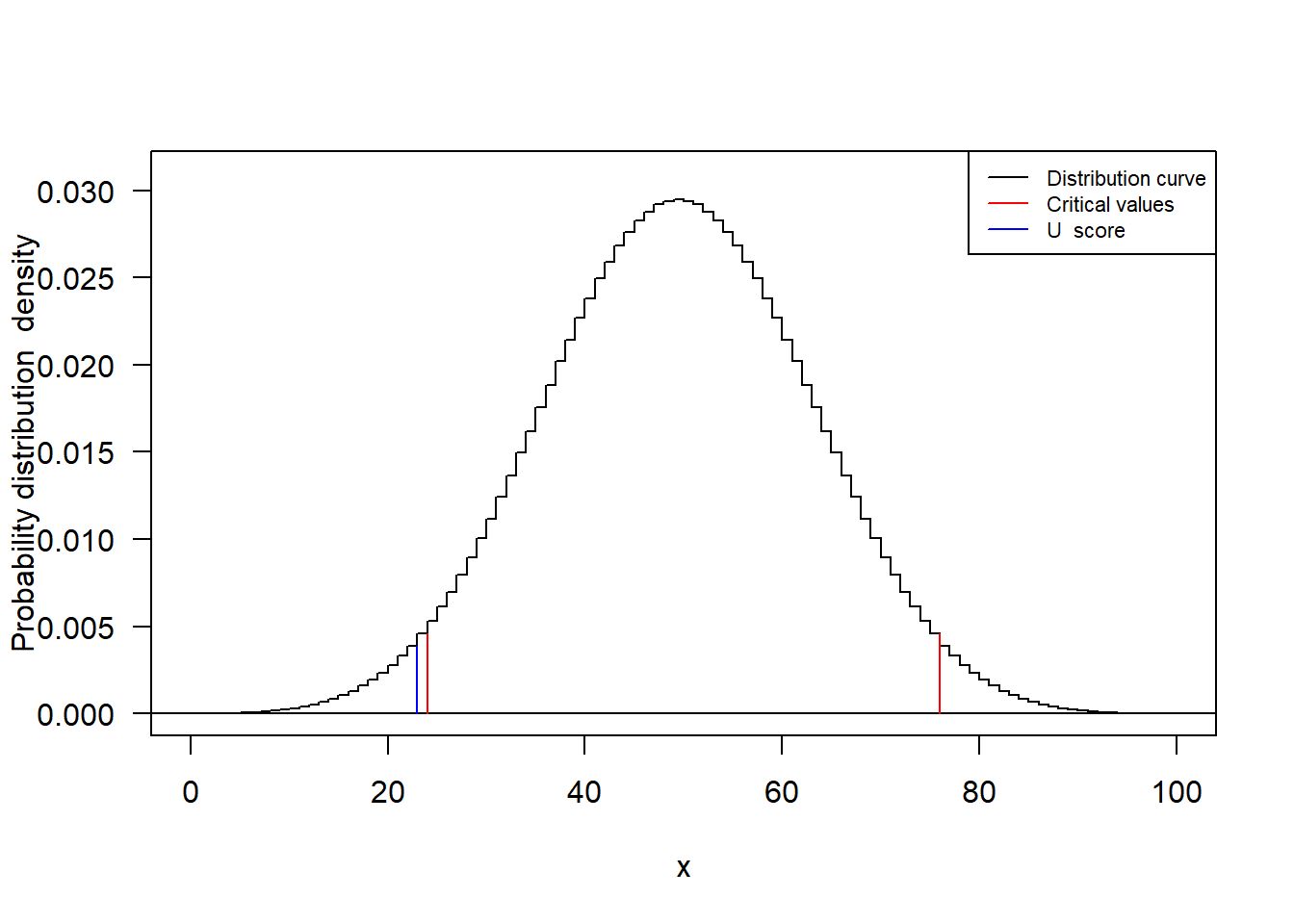
9.
The P-value is 0.043
dtf <- data.frame(City_A = c(13.31, 13.67, 12.805, 13.1, 13.39, 12.375, 11.58, 14.58, 12.029, 13.69),
                  City_B = c(14.14, 12.54, 15.63, 13.66, 15.51, 13.23, 13.25, 15.2, 14.18, 14.53))
test <- wilcox.test(dtf$City_A, dtf$City_B, conf.int=TRUE)
round(test$p.value, 3)
[1] 0.04310.
The P-value is smaller than 0.05, reject the H0 hypotheses.
11.
The two dataset medians are different at alpha=0.05. The City_A and City_B have significant different with the median PM2.5 concentrations.
12.
The mean and standard deviation of the approximate normal distribution are 50 and 13.22876
U_mu <- m * n / 2
U_mu
[1] 50U_sd <- sqrt(m * n * (m + n + 1) / 12)
U_sd[1] 13.2287613.
curve(dnorm(x, U_mu, U_sd), from=0, to=110)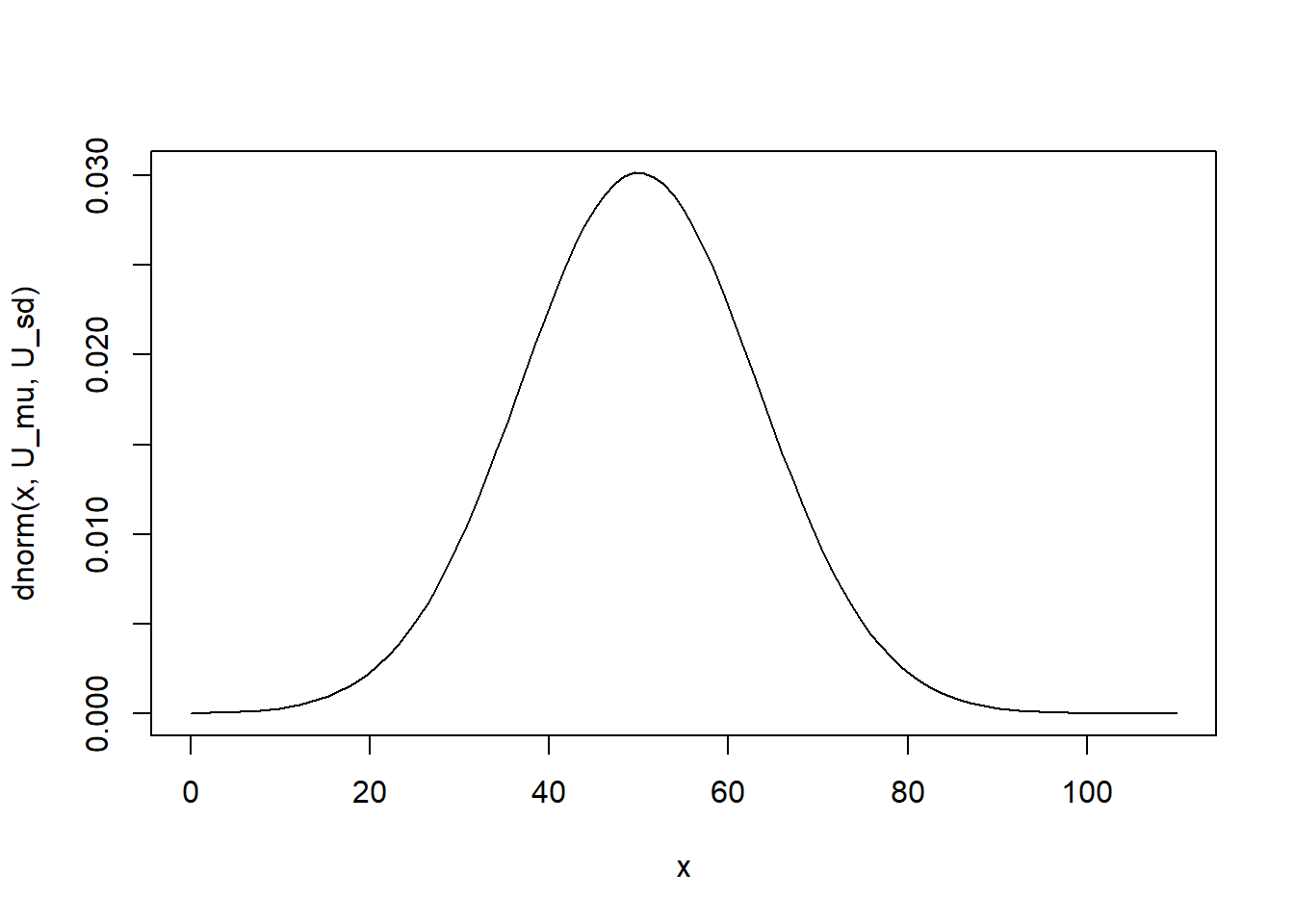
NA
NA
Sys.time()[1] "2023-05-11 12:27:12 CST"format(Sys.Date(), format = '%Y, %B, %d, %A')[1] "2023, May, 11, Thursday"t1 <- Sys.time()
t2 <- strptime( "2022-9-13 15:00:00", format="%Y-%m-%d %H:%M:%S" )
difftime(time1 = t1, time2 = t2, units = 'secs')Time difference of 20726833 secsdifftime(time1 = t1, time2 = t2, units = 'days')Time difference of 239.8939 daysdifftime(time1 = t1, time2 = t2, units = 'hours')Time difference of 5757.454 hourst3 <- as.Date( "9/13/2023", format="%m/%d/%Y" )
format(t3, format="%A")[1] "Wednesday"t4 <- as.Date( "9/13/2024", format="%m/%d/%Y" )
format(t4, format="%A")[1] "Friday"dates <- seq(as.Date("2020-09-13"), as.Date("2040-09-13"), by="year")
weekdays <- factor(weekdays(dates, abbreviate=TRUE),
levels=c("Sun", "Mon", "Tue", "Wed", "Thu", "Fri", "Sat"))
weekdays <- as.integer(format(dates, "%u"))
plot(weekdays, as.Date(dates, format="%Y" ),
xlab="Weekday", ylab="Year", main="September 13th, 2020-2040")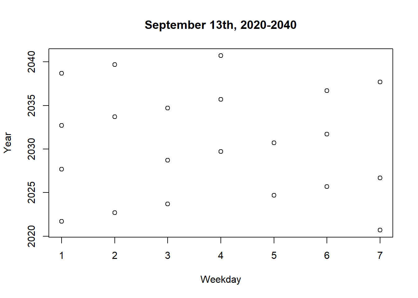
air<-read.csv("data/airquality.csv")
day <- paste("2022-",air$Month,"-",air$Day,sep="")
air$Date <- as.Date(day, format="%Y-%m-%d")air1<-na.omit(air)
subsets <- split(air1, air1$Month)
plots <- lapply(subsets, function(subset) {
plot(subset$Day, subset$Ozone,ylab = "Ozone pbb" ,main = paste("Ozone, ", unique(subset$Month))
)})
par(mfrow = c(2, 3))
for (i in seq_along(plots)) {
plot(plots[[i]])
}
library(ggthemes)
library(latex2exp)
dtf <- airquality
dtf5 <- dtf %>% subset(Date < "1973-06-01")
ggplot(dtf5) +
geom_point(aes(x = Date, y = Ozone))+
labs(y = "Ozone (ppb)") +
theme_classic() +
theme(axis.text.x = element_text(angle = 45, hjust = 1))
ggplot(dtf5) +
geom_point(aes(x = Date, y = Solar.R))+
labs(y = TeX("$\\text{Solar Radiation } (W\\cdot m^{-2})$")) +
theme_classic() +
theme(axis.text.x = element_text(angle = 45, hjust = 1))
ggplot(dtf5) +
geom_point(aes(x = Date, y = Wind))+
labs(y = TeX("$\\text{Wind speed }m\\cdot m^{-1}$")) +
theme_classic() +
theme(axis.text.x = element_text(angle = 45, hjust = 1))
ggplot(dtf5) +
geom_point(aes(x = Date, y = Temp))+
labs(y = TeX("$\\text{Temperature }\\circ C$")) +
theme_classic() +
theme(axis.text.x = element_text(angle = 45, hjust = 1))# install.packages("lubridate")
library(lubridate)
dtf$Weekday <- wday(as.Date(dtf$Date), week_start = 1)air1<-na.omit(air)
tapply(as.numeric(air1$Ozone),air1$Weekday,mean)
library(tidyverse)
mean_dtf <- dtf %>%
drop_na() %>%
group_by(Weekday) %>%
summarise(Ozone = mean(Ozone),
Solar.R = mean(Solar.R),
Wind = mean(Wind),
Temp = mean(Temp))library(latex2exp)
library(patchwork)
mean_ozone <- ggplot(mean_dtf) +
geom_line(aes(x = Weekday, y = Ozone)) +
labs(y = "Ozone (ppb)") +
theme_classic()
mean_solar <- ggplot(mean_dtf) +
geom_line(aes(x = Weekday, y = Solar.R)) +
labs(y = TeX("$\\text{Solar Radiation } (W\\cdot m^{-2})$")) +
theme_classic()
mean_wind <- ggplot(mean_dtf) +
geom_line(aes(x = Weekday, y = Wind))+
labs(y = TeX("$\\text{Wind speed }m\\cdot m^{-1}$")) +
theme_classic()
mean_temp <- ggplot(mean_dtf) +
geom_line(aes(x = Weekday, y = Temp))+
labs(y = TeX("$\\text{Temperature }\\circ C$")) +
theme_classic()setwd("data/smartflux/") # Remeber to delete the first file
temp <- list.files() %>%
substr(start = 1, stop =10) %>%
strptime(format = "%Y-%m-%d") %>%
format("%Y-%m-%d")
missing_files <- 0
for(i in 1:(length(temp)-1)){
diff <- as.vector(difftime(temp[i+1], temp[i], units = "days"))
if(diff != 1){
missing_files <- missing_files + diff -1
}
}
print(missing_files)
temp <- list.files()
files <- lapply(temp, function(i){
read.table(i, fill = TRUE)
})
missing_records <- 0
for(i in 1:length(files)){
records <- length(files[[i]][3:nrow(files[[i]]),4])
missing_records <- missing_records + 48 - records
}
missing_records <- missing_records + 48 * missing_files
print(missing_records)
library(latex2exp)
plot(iris$Sepal.Length, iris$Petal.Length, pch = 16, las = 1,
     xlab = TeX('D$_p$($\\mu$m)'),
     ylab = expression(frac('dN', 'dlogD'[p] * '(cm' ^-3 * ')')))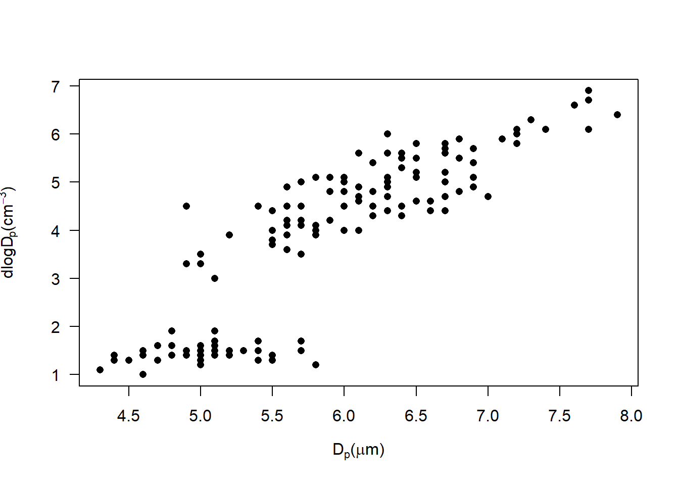
mymat <- matrix(c(1, 2, 3, 4), nrow = 2)
layout(mymat, widths = c(1, 2, 3, 2), heights = c(2, 1, 1, 2))
plot(co2)
plot(co2)
plot(co2)
plot(co2)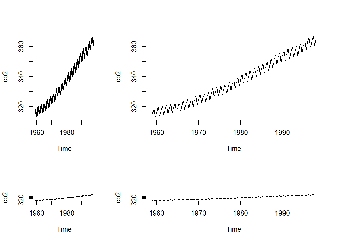
stocks <- data.frame(year   = c(2015, 2015, 2016, 2016),
                     half   = c(   1,    2,    1,    2),
                     return = c(1.88, 0.59, 0.92, 0.17))
stocks_wide <- stocks %>%
  pivot_wider(names_from = half, values_from = return)
stocks_wide
# A tibble: 2 × 3
year `1` `2`
<dbl> <dbl> <dbl>
1 2015 1.88 0.59
2 2016 0.92 0.17# because the column names 1999 and 2000 are not being correctly referenced.
table4a %>%
pivot_longer(c(`1999`, `2000`), names_to = "year", values_to = "cases")# A tibble: 6 × 3
country year cases
<chr> <chr> <dbl>
1 Afghanistan 1999 745
2 Afghanistan 2000 2666
3 Brazil 1999 37737
4 Brazil 2000 80488
5 China 1999 212258
6 China 2000 213766# Because there are duplicate values(columns) in the name and names columns (Not tidy)
people <- tribble(
~name, ~names, ~values,
"Phillip Woods", "age", 45,
"Phillip Woods", "height", 186,
"Phillip Woods", "age", 50,
"Jessica Cordero", "age", 37,
"Jessica Cordero", "height", 156
)preg <- tribble(
~pregnant, ~male, ~female,
"yes", NA, 10,
"no", 20, 12
)
preg1 <- pivot_longer(preg,c("male","female"),names_to = "Gender",values_to = "Number")
preg1# A tibble: 4 × 3
pregnant Gender Number
<chr> <chr> <dbl>
1 yes male NA
2 yes female 10
3 no male 20
4 no female 125.
(1) To determine which plane (tailnum) has the worst on-time record, we can calculate the average departure delay for each plane and then sort the results in ascending order to find the plane with the highest average delay.
# install.packages("nycflights13")
library(dplyr)
library(nycflights13)
flights %>%
  group_by(tailnum) %>%
  summarize(avg_dep_delay = mean(dep_delay, na.rm = TRUE)) %>%
  arrange(desc(avg_dep_delay)) %>%
  head(1)
# A tibble: 1 × 2
tailnum avg_dep_delay
<chr> <dbl>
1 N844MH 297
(2) We should depart at 5am, with a smallest time of dalay of 0.688 min on average.
flights %>%
  group_by(hour) %>%
  summarize(avg_dep_delay = mean(dep_delay, na.rm = TRUE)) %>%
  arrange(avg_dep_delay) %>%
  head(2)
# A tibble: 2 × 2
hour avg_dep_delay
<dbl> <dbl>
1 5 0.688
2 6 1.64
(3) To compute the total minutes of delay for each destination, we can group the flights by destination and calculate the total arrival and departure delays. And then we can add those two values together to get the total delay for each destination.
flights %>%
  group_by(dest) %>%
  summarise(total_delay = sum(arr_delay + dep_delay, na.rm = TRUE))
# A tibble: 105 × 2
dest total_delay
<chr> <dbl>
1 ABQ 4603
2 ACK 2983
3 ALB 15819
4 ANC 83
5 ATL 399462
6 AUS 45898
7 AVL 4216
8 BDL 10205
9 BGR 9732
10 BHM 12345
# ℹ 95 more rowsflights %>%
group_by(dest) %>%
mutate(total_delay = arr_delay + dep_delay) %>%
mutate(prop_delay = total_delay / sum(total_delay, na.rm = TRUE))# A tibble: 336,776 × 21
# Groups: dest [105]
year month day dep_time sched_dep_time dep_delay arr_time sched_arr_time
<int> <int> <int> <int> <int> <dbl> <int> <int>
1 2013 1 1 517 515 2 830 819
2 2013 1 1 533 529 4 850 830
3 2013 1 1 542 540 2 923 850
4 2013 1 1 544 545 -1 1004 1022
5 2013 1 1 554 600 -6 812 837
6 2013 1 1 554 558 -4 740 728
7 2013 1 1 555 600 -5 913 854
8 2013 1 1 557 600 -3 709 723
9 2013 1 1 557 600 -3 838 846
10 2013 1 1 558 600 -2 753 745
# ℹ 336,766 more rows
# ℹ 13 more variables: arr_delay <dbl>, carrier <chr>, flight <int>,
# tailnum <chr>, origin <chr>, dest <chr>, air_time <dbl>, distance <dbl>,
# hour <dbl>, minute <dbl>, time_hour <dttm>, total_delay <dbl>,
# prop_delay <dbl>(4)
(5) For each plane in each month, we can group the flights data by tailnum and month
flights %>%
  group_by(tailnum, month) %>%
  summarise(flights = n())
# A tibble: 37,988 × 3
# Groups: tailnum [4,044]
tailnum month flights
<chr> <int> <int>
1 D942DN 2 1
2 D942DN 3 2
3 D942DN 7 1
4 N0EGMQ 1 41
5 N0EGMQ 2 28
6 N0EGMQ 3 30
7 N0EGMQ 4 29
8 N0EGMQ 5 13
9 N0EGMQ 6 32
10 N0EGMQ 7 11
# ℹ 37,978 more rowslibrary(agricolae)
iris.aov <- aov(Sepal.Length ~ Species, data = iris)
summary(iris.aov) Df Sum Sq Mean Sq F value Pr(>F)
Species 2 63.21 31.606 119.3 <2e-16 ***
Residuals 147 38.96 0.265
---
Signif. codes: 0 '***' 0.001 '**' 0.01 '*' 0.05 '.' 0.1 ' ' 1LSD.test(iris.aov, "Species", console = TRUE)
Study: iris.aov ~ "Species"

LSD t Test for Sepal.Length

Mean Square Error:  0.2650082

Species,  means and individual ( 95 %) CI

           Sepal.Length       std  r      LCL      UCL Min Max
setosa            5.006 0.3524897 50 4.862126 5.149874 4.3 5.8
versicolor        5.936 0.5161711 50 5.792126 6.079874 4.9 7.0
virginica         6.588 0.6358796 50 6.444126 6.731874 4.9 7.9

Alpha: 0.05 ; DF Error: 147
Critical Value of t: 1.976233

least Significant Difference: 0.2034688

Treatments with the same letter are not significantly different.

           Sepal.Length groups
virginica         6.588      a
versicolor        5.936      b
setosa 5.006 cpairwise.t.test(iris$Sepal.Length, iris$Species, p.adjust.method = "bonferroni")
    Pairwise comparisons using t tests with pooled SD

data:  iris$Sepal.Length and iris$Species

           setosa  versicolor
versicolor 2.6e-15 -
virginica  < 2e-16 8.3e-09

P value adjustment method: bonferroni inflen <- data.frame("HTC"= c(38, 40, 32, 36, 40, 40, 38, 40, 38, 40, 36, 40, 40, 35, 45,
56, 60, 50, 50, 50, 35, 40, 40, 55, 35,
40, 42, 38, 46, 36),
"Source" = c(rep("Control",15),
rep("Dushu",10),
rep("Jinji",5)))
wg_aov1 <- aov(HTC~Source, data = inflen)
summary(wg_aov1) Df Sum Sq Mean Sq F value Pr(>F)
Source 2 450.5 225.23 6.669 0.00443 **
Residuals 27 911.8 33.77
---
Signif. codes: 0 '***' 0.001 '**' 0.01 '*' 0.05 '.' 0.1 ' ' 1summary(LSD.test(wg_aov1, "Source", alpha = 0.01,console = T))
Study: wg_aov1 ~ "Source"

LSD t Test for HTC

Mean Square Error:  33.7716

Source,  means and individual ( 99 %) CI

             HTC      std  r      LCL      UCL Min Max
Control 38.53333 2.996824 15 34.37598 42.69069  32  45
Dushu   47.10000 8.987028 10 42.00830 52.19170  35  60
Jinji   40.40000 3.847077  5 33.19925 47.60075  36  46

Alpha: 0.01 ; DF Error: 27
Critical Value of t: 2.770683

Groups according to probability of means differences and alpha level( 0.01 )

Treatments with the same letter are not significantly different.

             HTC groups
Dushu   47.10000      a
Jinji   40.40000     ab
Control 38.53333      b
Length Class Mode
statistics 4 data.frame list
parameters 5 data.frame list
means 10 data.frame list
comparison 0 -none- NULL
groups 2 data.frame listinflen_pt <- pairwise.t.test(inflen$HTC, inflen$Source, pool.sd = FALSE,var.equal = TRUE, p.adj = "bonferroni")
inflen_pt
    Pairwise comparisons using t tests with non-pooled SD

data:  inflen$HTC and inflen$Source

      Control Dushu
Dushu 0.0066  -
Jinji 0.8227  0.4191

P value adjustment method: bonferroni inflen_pt$p.value < 0.01 Control Dushu
Dushu TRUE NA
Jinji FALSE FALSEWilcoxon Rank-Sum test: Used to compare whether the medians of two independent groups are equal. It is suitable for situations where the sample does not follow a normal distribution or where the variances are unequal.
Wilcoxon Signed-Rank test: Used to compare whether the medians of two related groups are equal. It is suitable for situations where the sample does not follow a normal distribution or where the variances are unequal.
Kruskal-Wallis test: Used to compare whether the medians of three or more independent groups are equal. It is suitable for situations where the sample does not follow a normal distribution or where the variances are unequal.
Friedman test: Used to compare whether the medians of three or more related groups are equal. It is suitable for situations where the sample does not follow a normal distribution or where the variances are unequal.
dtf <- read.csv('data/tce.csv')
wilcox.test(dtf$TCE.mg.per.L[dtf$Period == 'Before'],
            dtf$TCE.mg.per.L[dtf$Period == 'After'],
            paired = TRUE, conf.int = TRUE,
            correct = FALSE)
    Wilcoxon signed rank exact test

data:  dtf$TCE.mg.per.L[dtf$Period == "Before"] and dtf$TCE.mg.per.L[dtf$Period == "After"]
V = 55, p-value = 0.001953
alternative hypothesis: true location shift is not equal to 0
95 percent confidence interval:
  6.8650 28.5715
sample estimates:
(pseudo)median
18.78 kruskal.test(Sepal.Length ~ Species, data = iris)
    Kruskal-Wallis rank sum test

data:  Sepal.Length by Species
Kruskal-Wallis chi-squared = 96.937, df = 2, p-value < 2.2e-16boxplot(Sepal.Length ~ Species,
data = iris,
horizontal = TRUE,
notch = TRUE, las = 1)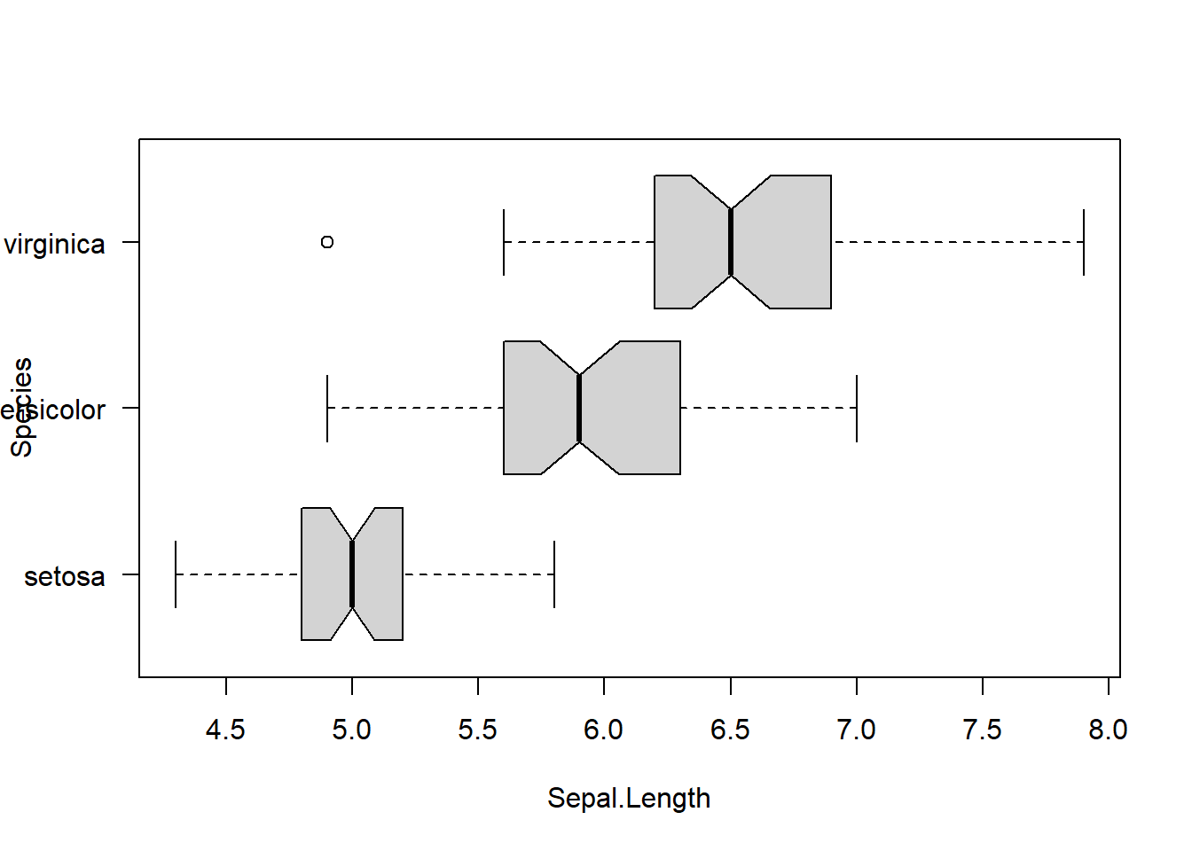
# Step 1: Visualization
dtf <- airquality[, -6]
dtf <- na.omit(dtf)
dtf_cor <- cor(dtf)
GGally::ggpairs(dtf)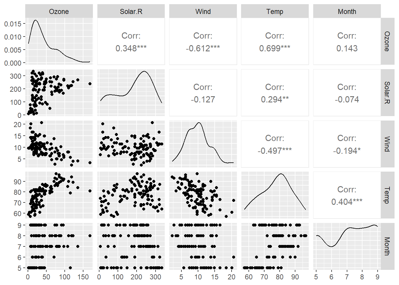
pairs(dtf)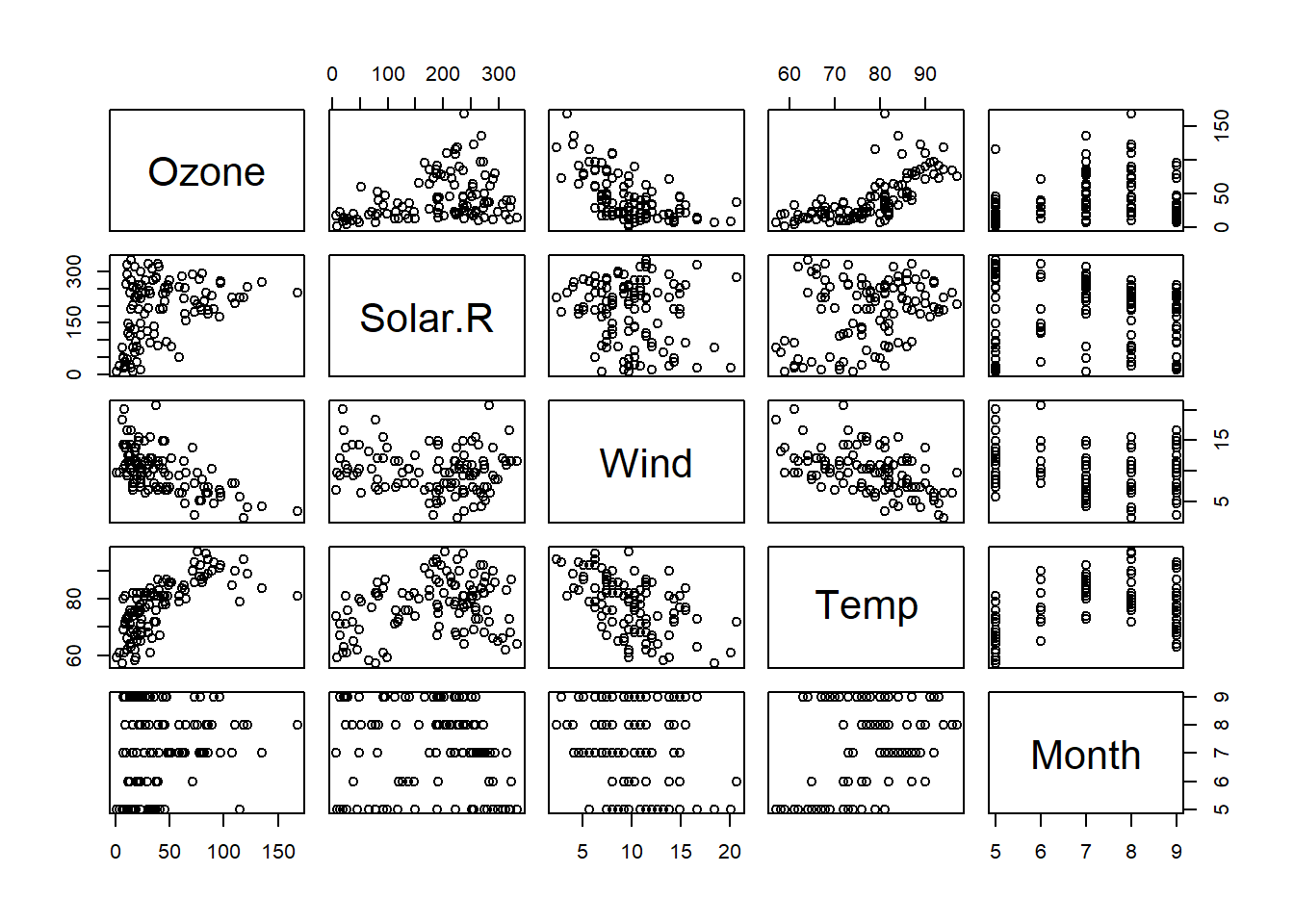
corrplot::corrplot(dtf_cor,
                   order = 'AOE',
                   type = "upper",
                   method = "number")
corrplot::corrplot(dtf_cor,
                   order = "AOE",
                   type = "lower",
                   method = "ell",
                   diag = FALSE,
                   tl.pos = "l",
                   cl.pos = "n",
                   add = TRUE)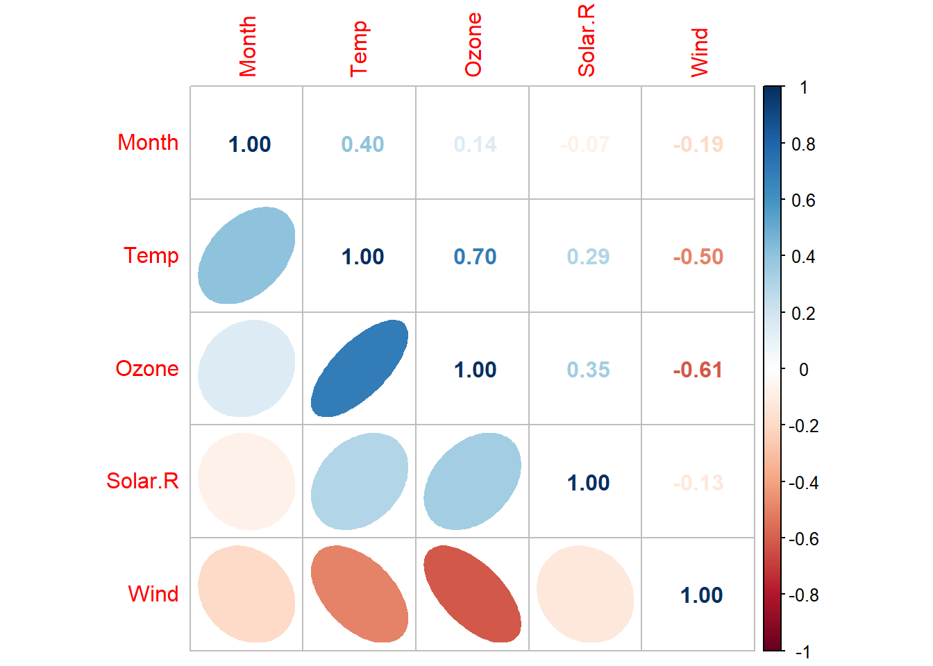
# Step 2: Maximal model
ozone_concentration_lm <- lm(Ozone ~ ., data = dtf)
summary(ozone_concentration_lm)
Call:
lm(formula = Ozone ~ ., data = dtf)

Residuals:
    Min      1Q  Median      3Q     Max
-35.870 -13.968  -2.671   9.553  97.918

Coefficients:
             Estimate Std. Error t value Pr(>|t|)
(Intercept) -58.05384   22.97114  -2.527   0.0130 *
Solar.R       0.04960    0.02346   2.114   0.0368 *
Wind         -3.31651    0.64579  -5.136 1.29e-06 ***
Temp          1.87087    0.27363   6.837 5.34e-10 ***
Month        -2.99163    1.51592  -1.973   0.0510 .
---
Signif. codes:  0 '***' 0.001 '**' 0.01 '*' 0.05 '.' 0.1 ' ' 1

Residual standard error: 20.9 on 106 degrees of freedom
Multiple R-squared:  0.6199,    Adjusted R-squared:  0.6055
F-statistic: 43.21 on 4 and 106 DF, p-value: < 2.2e-16confint(ozone_concentration_lm) 2.5 % 97.5 %
(Intercept) -1.035964e+02 -12.51131722
Solar.R 3.088529e-03 0.09610512
Wind -4.596849e+00 -2.03616955
Temp 1.328372e+00 2.41337586
Month -5.997092e+00 0.01383629anova(ozone_concentration_lm)Analysis of Variance Table
Response: Ozone
Df Sum Sq Mean Sq F value Pr(>F)
Solar.R 1 14780 14780 33.8357 6.427e-08 ***
Wind 1 39969 39969 91.5037 5.327e-16 ***
Temp 1 19050 19050 43.6117 1.639e-09 ***
Month 1 1701 1701 3.8946 0.05104 .
Residuals 106 46302 437
---
Signif. codes: 0 '***' 0.001 '**' 0.01 '*' 0.05 '.' 0.1 ' ' 1# Step 3: Check the Multicollinearity
faraway::vif(dtf[, -1]) Solar.R Wind Temp Month
1.151409 1.329309 1.712455 1.256371 # Step 4: simplify the model using Backward selection
get_p <- function(model){
smry2 <- data.frame(summary(model)$coefficients)
smry2[order(-smry2$Pr...t..), ]
}
get_p(ozone_concentration_lm) Estimate Std..Error t.value Pr...t..
Month -2.99162786 1.51592267 -1.973470 5.104492e-02
Solar.R 0.04959683 0.02345827 2.114258 3.683836e-02
(Intercept) -58.05383883 22.97114118 -2.527251 1.297198e-02
Wind -3.31650940 0.64578918 -5.135591 1.286145e-06
Temp 1.87087379 0.27363201 6.837189 5.337230e-10lm2 <- update(ozone_concentration_lm,.~.-Month)
get_p(lm2) Estimate Std..Error t.value Pr...t..
Solar.R 0.05982059 0.02318647 2.579979 1.123664e-02
(Intercept) -64.34207893 23.05472435 -2.790841 6.226638e-03
Wind -3.33359131 0.65440710 -5.094063 1.515934e-06
Temp 1.65209291 0.25352979 6.516366 2.423506e-09lm3 <- step(ozone_concentration_lm, direction = "both")Start: AIC=679.71
Ozone ~ Solar.R + Wind + Temp + Month
Df Sum of Sq RSS AIC
<none> 46302 679.71
- Month 1 1701.2 48003 681.71
- Solar.R 1 1952.6 48254 682.29
- Wind 1 11520.5 57822 702.37
- Temp 1 20419.5 66721 718.26# Step 5: report the results
summary(lm2)
Call:
lm(formula = Ozone ~ Solar.R + Wind + Temp, data = dtf)

Residuals:
    Min      1Q  Median      3Q     Max
-40.485 -14.219  -3.551  10.097  95.619

Coefficients:
             Estimate Std. Error t value Pr(>|t|)
(Intercept) -64.34208   23.05472  -2.791  0.00623 **
Solar.R       0.05982    0.02319   2.580  0.01124 *
Wind         -3.33359    0.65441  -5.094 1.52e-06 ***
Temp          1.65209    0.25353   6.516 2.42e-09 ***
---
Signif. codes:  0 '***' 0.001 '**' 0.01 '*' 0.05 '.' 0.1 ' ' 1

Residual standard error: 21.18 on 107 degrees of freedom
Multiple R-squared:  0.6059,    Adjusted R-squared:  0.5948
F-statistic: 54.83 on 3 and 107 DF, p-value: < 2.2e-16stargazer::stargazer(lm2, type = 'text')
===============================================
                        Dependent variable:
                    ---------------------------
                               Ozone
-----------------------------------------------
Solar.R                       0.060**
                              (0.023)

Wind                         -3.334***
                              (0.654)

Temp                         1.652***
                              (0.254)

Constant                    -64.342***
                             (23.055)

-----------------------------------------------
Observations                    111
R2                             0.606
Adjusted R2                    0.595
Residual Std. Error      21.181 (df = 107)
F Statistic           54.834*** (df = 3; 107)
===============================================
Note: *p<0.1; **p<0.05; ***p<0.01dtf <- read.csv("data/heart.data.csv")
dtf <- dtf[, -1]
dtf <- na.omit(dtf)
dtf_cor <- cor(dtf)
GGally::ggpairs(dtf)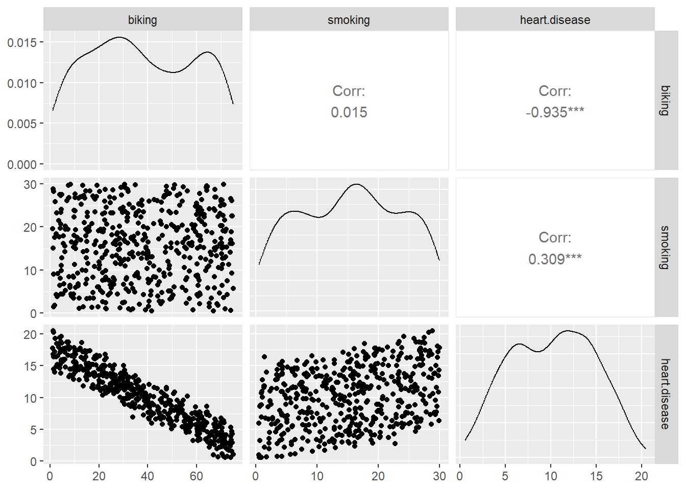
corrplot::corrplot(dtf_cor,
                   order = 'AOE',
                   type = "upper",
                   method = "number")
corrplot::corrplot(dtf_cor,
                   order = "AOE",
                   type = "lower",
                   method = "ell",
                   diag = FALSE,
                   tl.pos = "l",
                   cl.pos = "n",
                   add = TRUE)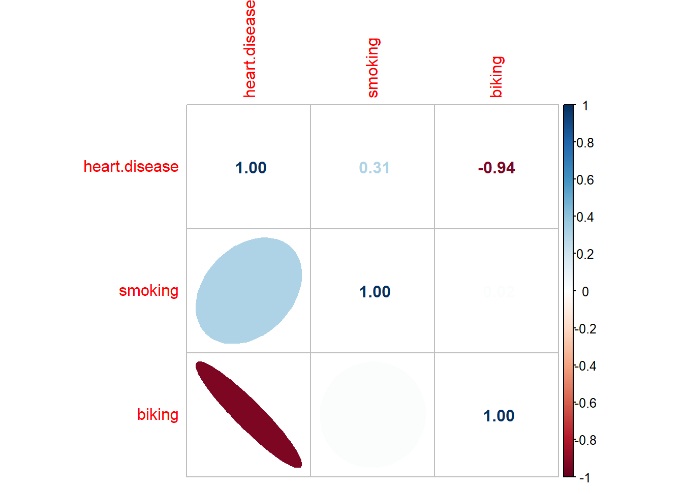
heart_disease_lm <- lm(heart.disease ~ ., data = dtf)
summary(heart_disease_lm)
Call:
lm(formula = heart.disease ~ ., data = dtf)

Residuals:
    Min      1Q  Median      3Q     Max
-2.1789 -0.4463  0.0362  0.4422  1.9331

Coefficients:
             Estimate Std. Error t value Pr(>|t|)
(Intercept) 14.984658   0.080137  186.99   <2e-16 ***
biking      -0.200133   0.001366 -146.53   <2e-16 ***
smoking      0.178334   0.003539   50.39   <2e-16 ***
---
Signif. codes:  0 '***' 0.001 '**' 0.01 '*' 0.05 '.' 0.1 ' ' 1

Residual standard error: 0.654 on 495 degrees of freedom
Multiple R-squared:  0.9796,    Adjusted R-squared:  0.9795
F-statistic: 1.19e+04 on 2 and 495 DF, p-value: < 2.2e-16confint(heart_disease_lm) 2.5 % 97.5 %
(Intercept) 14.8272075 15.1421084
biking -0.2028166 -0.1974495
smoking 0.1713800 0.1852878anova(heart_disease_lm)Analysis of Variance Table
Response: heart.disease
Df Sum Sq Mean Sq F value Pr(>F)
biking 1 9090.6 9090.6 21251.7 < 2.2e-16 ***
smoking 1 1086.0 1086.0 2538.8 < 2.2e-16 ***
Residuals 495 211.7 0.4
---
Signif. codes: 0 '***' 0.001 '**' 0.01 '*' 0.05 '.' 0.1 ' ' 1faraway::vif(dtf[, 1:2]) biking smoking
1.000229 1.000229 get_p <- function(model){
smry2 <- data.frame(summary(model)$coefficients)
smry2[order(-smry2$Pr...t..), ]
}
get_p(heart_disease_lm) Estimate Std..Error t.value Pr...t..
smoking 0.1783339 0.003539307 50.38667 5.192235e-197
(Intercept) 14.9846580 0.080136914 186.98821 0.000000e+00
biking -0.2001331 0.001365858 -146.52547 0.000000e+00stargazer::stargazer(heart_disease_lm, type = 'text')
===============================================
                        Dependent variable:
                    ---------------------------
                           heart.disease
-----------------------------------------------
biking                       -0.200***
                              (0.001)

smoking                      0.178***
                              (0.004)

Constant                     14.985***
                              (0.080)

-----------------------------------------------
Observations                    498
R2                             0.980
Adjusted R2                    0.980
Residual Std. Error      0.654 (df = 495)
F Statistic         11,895.240*** (df = 2; 495)
===============================================
Note: *p<0.1; **p<0.05; ***p<0.01To be continue…
A scientist studies the effect of seizure drugs on the number of seizures during the first eight weeks of treatment. The dataset is available in the robust package:
Carry out a Poisson regression of the number of seizures after treatment (sumY) as the dependent variable, and the treatment conditions (Trt), Age, and the number of seizures before treatment (Base) as the independent variables.
data("breslow.dat", package = 'robust')
View(breslow.dat)

fit.breslow <- glm(sumY ~ Trt + Age + Base, data = breslow.dat, family = poisson())
summary(fit.breslow)
Call:
glm(formula = sumY ~ Trt + Age + Base, family = poisson(), data = breslow.dat)

Deviance Residuals:
    Min       1Q   Median       3Q      Max
-6.0569  -2.0433  -0.9397   0.7929  11.0061

Coefficients:
               Estimate Std. Error z value Pr(>|z|)
(Intercept)   1.9488259  0.1356191  14.370  < 2e-16 ***
Trtprogabide -0.1527009  0.0478051  -3.194   0.0014 **
Age           0.0227401  0.0040240   5.651 1.59e-08 ***
Base          0.0226517  0.0005093  44.476  < 2e-16 ***
---
Signif. codes:  0 '***' 0.001 '**' 0.01 '*' 0.05 '.' 0.1 ' ' 1

(Dispersion parameter for poisson family taken to be 1)

    Null deviance: 2122.73  on 58  degrees of freedom
Residual deviance:  559.44  on 55  degrees of freedom
AIC: 850.71

Number of Fisher Scoring iterations: 5exp(coef(fit.breslow)) (Intercept) Trtprogabide Age Base
7.0204403 0.8583864 1.0230007 1.0229102 stargazer::stargazer(fit.breslow, type = 'text')
=============================================
                      Dependent variable:
                  ---------------------------
                             sumY
---------------------------------------------
Trtprogabide               -0.153***
                            (0.048)

Age                        0.023***
                            (0.004)

Base                       0.023***
                            (0.001)

Constant                   1.949***
                            (0.136)

---------------------------------------------
Observations                  59
Log Likelihood             -421.354
Akaike Inf. Crit.           850.707
=============================================
Note: *p<0.1; **p<0.05; ***p<0.01equatiomatic::extract_eq(fit.breslow, use_coefs = TRUE)\[ \log ({ \widehat{E( \operatorname{sumY} )} }) = 1.95 - 0.15(\operatorname{Trt}_{\operatorname{progabide}}) + 0.02(\operatorname{Age}) + 0.02(\operatorname{Base}) \]
fit.breslow.od <- glm(sumY ~ Trt + Age + Base, data = breslow.dat, family = quasipoisson())
summary(fit.breslow.od)
Call:
glm(formula = sumY ~ Trt + Age + Base, family = quasipoisson(),
    data = breslow.dat)

Deviance Residuals:
    Min       1Q   Median       3Q      Max
-6.0569  -2.0433  -0.9397   0.7929  11.0061

Coefficients:
              Estimate Std. Error t value Pr(>|t|)
(Intercept)   1.948826   0.465091   4.190 0.000102 ***
Trtprogabide -0.152701   0.163943  -0.931 0.355702
Age           0.022740   0.013800   1.648 0.105085
Base          0.022652   0.001747  12.969  < 2e-16 ***
---
Signif. codes:  0 '***' 0.001 '**' 0.01 '*' 0.05 '.' 0.1 ' ' 1

(Dispersion parameter for quasipoisson family taken to be 11.76075)

    Null deviance: 2122.73  on 58  degrees of freedom
Residual deviance:  559.44  on 55  degrees of freedom
AIC: NA

Number of Fisher Scoring iterations: 5exp(coef(fit.breslow.od)) (Intercept) Trtprogabide Age Base
7.0204403 0.8583864 1.0230007 1.0229102 stargazer::stargazer(fit.breslow.od, type = 'text')
========================================
                 Dependent variable:
             ---------------------------
                        sumY
----------------------------------------
Trtprogabide           -0.153
                       (0.164)

Age                     0.023
                       (0.014)

Base                  0.023***
                       (0.002)

Constant              1.949***
                       (0.465)

----------------------------------------
Observations             59
========================================
Note: *p<0.1; **p<0.05; ***p<0.01equatiomatic::extract_eq(fit.breslow.od, use_coefs = TRUE)\[ \log ({ \widehat{E( \operatorname{sumY} )} }) = 1.95 - 0.15(\operatorname{Trt}_{\operatorname{progabide}}) + 0.02(\operatorname{Age}) + 0.02(\operatorname{Base}) \]
R version 4.2.3 (2023-03-15 ucrt)
Platform: x86_64-w64-mingw32/x64 (64-bit)
Running under: Windows 10 x64 (build 19044)

Matrix products: default

locale:
[1] LC_COLLATE=Chinese (Simplified)_China.utf8
[2] LC_CTYPE=Chinese (Simplified)_China.utf8
[3] LC_MONETARY=Chinese (Simplified)_China.utf8
[4] LC_NUMERIC=C
[5] LC_TIME=English_United States.1252

attached base packages:
[1] stats     graphics  grDevices utils     datasets  methods   base

other attached packages:
 [1] agricolae_1.3-5    nycflights13_1.0.2 lubridate_1.9.2    forcats_1.0.0
 [5] stringr_1.5.0      purrr_1.0.1        readr_2.1.4        tidyr_1.3.0
 [9] tibble_3.2.1       ggplot2_3.4.2      tidyverse_2.0.0    openair_2.16-0
[13] dplyr_1.1.0        latex2exp_0.9.6

loaded via a namespace (and not attached):
 [1] nlme_3.1-162        RColorBrewer_1.1-3  backports_1.4.1
 [4] tools_4.2.3         utf8_1.2.3          R6_2.5.1
 [7] AlgDesign_1.2.1     mgcv_1.8-42         questionr_0.7.8
[10] colorspace_2.1-0    withr_2.5.0         tidyselect_1.2.0
[13] GGally_2.1.2        klaR_1.7-2          compiler_4.2.3
[16] cli_3.6.1           labeling_0.4.2      equatiomatic_0.3.1
[19] scales_1.2.1        hexbin_1.28.3       digest_0.6.31
[22] minqa_1.2.5         rmarkdown_2.21      jpeg_0.1-10
[25] pkgconfig_2.0.3     htmltools_0.5.4     lme4_1.1-31
[28] labelled_2.11.0     fastmap_1.1.0       highr_0.10
[31] maps_3.4.1          htmlwidgets_1.6.2   rlang_1.1.0
[34] rstudioapi_0.14     shiny_1.7.4         generics_0.1.3
[37] farver_2.1.1        combinat_0.0-8      jsonlite_1.8.4
[40] magrittr_2.0.3      interp_1.1-4        Matrix_1.5-3
[43] Rcpp_1.0.10         munsell_0.5.0       fansi_1.0.3
[46] lifecycle_1.0.3     stringi_1.7.12      yaml_2.3.7
[49] MASS_7.3-58.2       plyr_1.8.8          grid_4.2.3
[52] promises_1.2.0.1    miniUI_0.1.1.1      deldir_1.0-6
[55] lattice_0.20-45     stargazer_5.2.3     haven_2.5.2
[58] splines_4.2.3       mapproj_1.2.11      hms_1.1.3
[61] knitr_1.42          pillar_1.9.0        boot_1.3-28.1
[64] glue_1.6.2          evaluate_0.20       latticeExtra_0.6-30
[67] nloptr_2.0.3        png_0.1-8           vctrs_0.6.2
[70] tzdb_0.3.0          httpuv_1.6.9        gtable_0.3.3
[73] reshape_0.8.9       xfun_0.37           mime_0.12
[76] broom_1.0.4         xtable_1.8-4        later_1.3.0
[79] faraway_1.0.8       cluster_2.1.4       corrplot_0.92
[82] timechange_0.2.0    ellipsis_0.3.2